The imperfect art of climate change modelling

The completed Group I report from the 5^th Intergovernmental Panel on Climate Change (IPCC) assessment was published in January (see previous post on summary report in September). One of the few definite statements made in the report was that “global mean temperatures will continue to rise over the 21st century if greenhouse gas (GHG) emissions continue unabat­ed”. How we measure the impact of such changes is therefore incredibly important. A recent article in the FT by Robin Harding on the topic which highlighted the shortcomings of models used to assess the impact of climate change therefore caught my attention.

The article referred to two academic papers, one by Robert Pindyck and another by Nicholas Stern, which contained damning criticism of models that integrate climate and economic models, so called integrated assessment models (IAM).

Pindyck states that “IAM based analyses of climate policy create a perception of knowledge and precision, but that perception is illusory and misleading”. Stern also criticizes IAMs stating that “assumptions built into the economic modelling on growth, damages and risks, come close to assuming directly that the impacts and costs will be modest and close to excluding the possibility of catastrophic outcomes”.

These comments remind me of Paul Wilmott, the influential English quant, who included in his Modeller’s Hippocratic Oath the following: “I will remember that I didn’t make the world, and it doesn’t satisfy my equations” (see Quotes section of this website for more quotes on models).

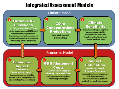
In his paper, Pindyck characterised the IAMs currently used into 6 core components as the graphic below illustrates.

click to enlarge

Pindyck highlights a number of the main elements of IAMs which involve a considerable amount of arbitrary choice, including climate sensitivity, the damage and social welfare (utility) functions. He cites important feedback loops in climates as difficult, if not impossible, to determine. Although there has been some good work in specific areas like agriculture, Pindyck is particularly critical on the damage functions, saying many are essentially made up. The final piece on social utility and the rate of time preference are essentially policy parameter which are open to political forces and therefore subject to considerable variability (& that’s a polite way of putting it).

The point about damage functions is an interesting one as these are also key determinants in the catastrophe vendor models widely used in the insurance sector. As a previous post on Florida highlighted, even these specific and commercially developed models result in varying outputs.

One example of IAMs directly influencing current policymakers is those used by the Interagency Working Group (IWG) which under the Obama administration is the entity that determines the social cost of carbon (SCC), defined as the net present damage done by emitting a marginal ton of CO₂ equivalent (CO₂e), used in regulating industries such as the petrochemical sector. Many IAMs are available (the sector even has its own journal – The Integrated Assessment Journal!) and the IWG relies on three of the oldest and most well know; the Dynamic Integrated Climate and Economy (DICE) model, the Policy Analysis of the Greenhouse Effect (PAGE) model, and the fun sounding Climate Framework for Uncertainty, Negotiation, and Distribution (FUND) model.

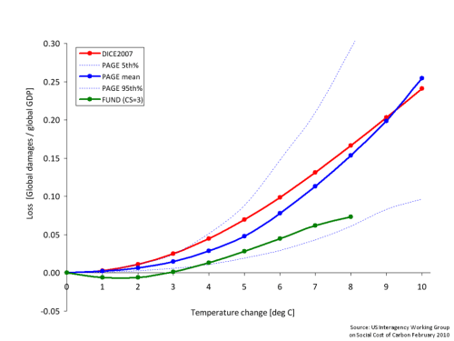
The first IWG paper in 2010 included an exhibit, reproduced below, summarizing the economic impact of raising temperatures based upon the 3 models.

click to enlarge

To be fair to the IWG, they do highlight that “underlying the three IAMs selected for this exercise are a number of simplifying assumptions and judgments reflecting the various modelers’ best attempts to synthesize the available scientific and economic research characterizing these relationships”.

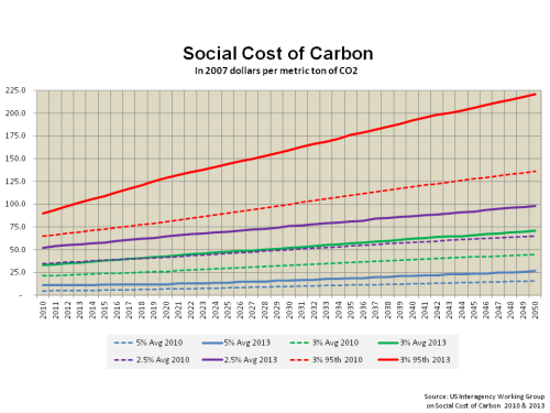
The IWG released an updated paper in 2013 whereby revised SCC estimates were presented based upon a number of amendments to the underlying models. Included in these changes are revisions to damage functions and to climate sensitivity assumptions. The results of the changes on average and 95^th percentile SCC estimates, at varying discount rates (which are obviously key determinants to the SCC given the long term nature of the impacts), can be clearly seen in the graph below.

click to enlarge

Given the magnitude of the SCC changes, it is not surprising that critics of the charges, including vested interests such as petrochemical lobbyists, are highlighting the uncertainty in IAMs as a counter against the charges. The climate change deniers love any opportunity to discredit the science as they demonstrated so ably with the 4^th IPCC assessment. The goal has to be to improve modelling as a risk management tool that results in sensible preventative measures. Pindyck emphasises that his criticisms should not be an excuse for inaction. He believes we should follow a risk management approach focused on the risk of catastrophe with models updated as more information emerges and uses the threat of nuclear oblivion during the Cold War as a parallel. He argues that “one can think of a GHG abatement policy as a form of insurance: society would be paying for a guarantee that a low-probability catastrophe will not occur (or is less likely)”. Stern too advises that our focus should be on potential extreme damage and that the economic community need to refocus and combine current insights where “an examination and modelling of ways in which disruption and decline can occur”.

Whilst I was looking into this subject, I took the time to look over the completed 5^th assessment report from the IPCC. First, it is important to stress that the IPCC acknowledge the array of uncertainties in predicting climate change. They state the obvious in that “the nonlinear and chaotic nature of the climate system imposes natu­ral limits on the extent to which skilful predictions of climate statistics may be made”. They assert that the use of multiple scenarios and models is the best way we have for determining “a wide range of possible future evolutions of the Earth’s climate”. They also accept that “predicting socioeconomic development is arguably even more difficult than predicting the evolution of a physical system”.

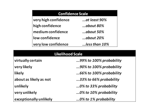
The report uses a variety of terms in its findings which I summarised in a previous post and reproduce below.

click to enlarge

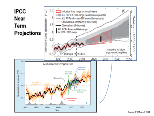
Under the medium term prediction section (Chapter 11) which covers the period 2016 to 2035 relative to the reference period 1986 to 2005, a number of the notable predictions include:

• The projected change in global mean surface air temperature will likely be in the range 0.3 to 0.7°C (medium confidence).
• It is more likely than not that the mean global mean surface air temperature for the period 2016–2035 will be more than 1°C above the mean for 1850–1900, and very unlikely that it will be more than 1.5°C above the 1850–1900 mean (medium confidence).
• Zonal mean precipitation will very likely increase in high and some of the mid-latitudes, and will more likely than not decrease in the subtropics. The frequency and intensity of heavy precipitation events over land will likely increase on average in the near term (this trend will not be apparent in all regions).
• It is very likely that globally averaged surface and vertically averaged ocean temperatures will increase in the near term. It is likely that there will be increases in salinity in the tropical and (especially) subtropical Atlantic, and decreases in the western tropical Pacific over the next few decades.
• In most land regions the frequency of warm days and warm nights will likely increase in the next decades, while that of cold days and cold nights will decrease.
• There is low confidence in basin-scale projections of changes in the intensity and frequency of tropical cyclones (TCs) in all basins to the mid-21st century and there is low confidence in near-term projections for increased TC intensity in the North Atlantic.

The last bullet point is especially interesting for the insurance sector involved in providing property catastrophe protection. Graphically I have reproduced two interesting projections below (Note: no volcano activity is assumed).

click to enlarge

Under the longer term projections in Chapter 12, the IPCC makes the definite statement that opened this post. It also states that it is virtually certain that, in most places, there will be more hot and fewer cold temperature extremes as global mean temper­atures increase and that, in the long term, global precipitation will increase with increased global mean surface temperature.

I don’t know about you but it seems to me a sensible course of action that we should be taking scenarios that the IPCC is predicting with virtual certainty and applying a risk management approach to how we can prepare for or counteract extremes as recommended by experts such as Pindyck and Stern.

The quote “it’s better to do something imperfectly than to do nothing perfectly” comes to mind. In this regard, for the sake of our children at the very least, we should embrace the imperfect art of climate change modelling and figure out how best to use them in getting things done.