Tag Archives: probability of default

Divine Diversification

There have been some interesting developments in the US insurance sector on the issue of systemically important financial institutions (SIFIs). Metlife announced plans to separate some of their US life retail units to avoid the designation whilst shareholder pressure is mounting on AIG to do the same. These events are symptoms of global regulations designed to address the “too big to fail” issue through higher capital requirements. It is interesting however that these regulations are having an impact in the insurance sector rather than the more impactful issue within the banking sector (this may have to do with the situation where the larger banks will retain their SIFI status unless the splits are significant).

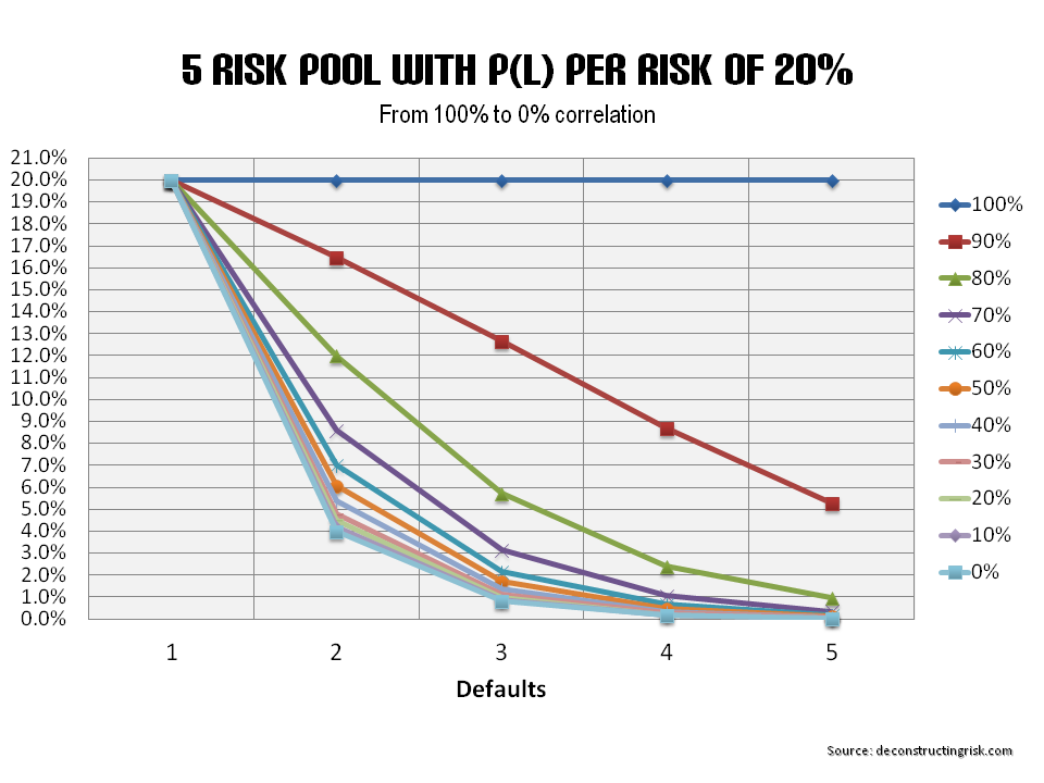
The developments also fly in the face of the risk management argument articulated by the insurance industry that diversification is the answer to the ills of failure. This is the case AIG are arguing to counter calls for a breakup. Indeed, the industry uses the diversification of risk in their defences against the sector being deemed of systemic import, as the exhibit below from a report on systemic risk in insurance from an industry group, the Geneva Association, in 2010 illustrates. Although the point is often laboured by the insurance sector (there still remains important correlations between each of the risk types), the graph does make a valid point.

click to enlargeEconomic Capital Breakdown for European Banks and Insurers

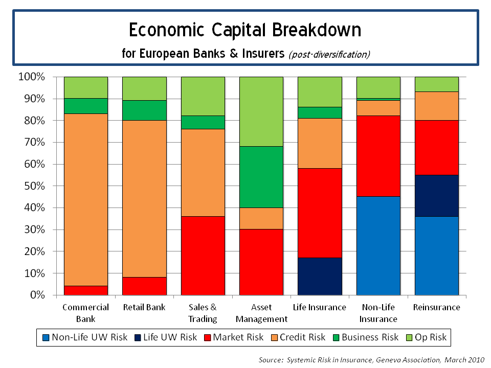
The 1st of January this year marked the introduction of the new Solvency II regulatory regime for insurers in Europe, some 15 years after work begun on the new regime. The new risk based solvency regime allows insurers to use their own internal models to calculate their required capital and to direct their risk management framework. A flurry of internal model approvals by EU regulators were announced in the run-up to the new year, although the amount of approvals was far short of that anticipated in the years running up to January 2016. There will no doubt be some messy teething issues as the new regime is introduced. In a recent post, I highlighted the hoped for increased disclosures from European insurers on their risk profiles which will result from Solvency II. It is interesting that Fitch came out his week and stated that “Solvency II metrics are not comparable between insurers due to their different calculation approaches and will therefore not be a direct driver of ratings” citing issues such as the application of transitional measures and different regulator approaches to internal model approvals.

I have written many times on the dangers of overtly generous diversification benefits (here, here, here, and here are just a few!) and this post continues that theme. A number of the large European insurers have already published details of their internal model calculations in annual reports, investor and analyst presentations. The graphic below shows the results from 3 large insurers and 3 large reinsurers which again illustrate the point on diversification between risk types.

click to enlargeInternal Model Breakdown for European Insurers and Reinsurers

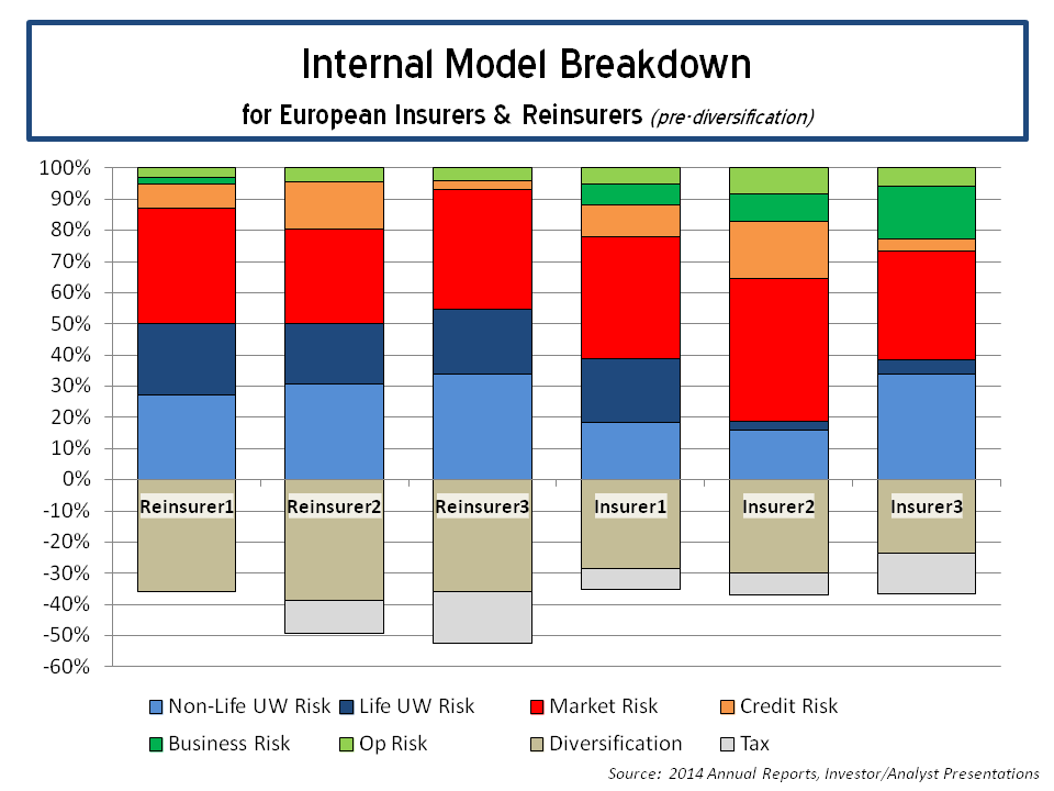
The reinsurers show, as one would expect, the largest diversification benefit between risk types (remember there is also significant diversification benefits assumed within risk types, more on that later) ranging from 35% to 40%. The insurers, depending upon business mix, only show between 20% and 30% diversification across risk types. The impact of tax offsets is also interesting with one reinsurer claiming a further 17% benefit! A caveat on these figures is needed, as Fitch points out; as different firms use differing terminology and methodology (credit risk is a good example of significant differences). I compared the diversification benefits assumed by these firms against what the figure would be using the standard formula correlation matrix and the correlations assuming total independence between the risk types (e.g. square root of the sum of squares), as below.

click to enlargeDiversification Levels within European Insurers and Reinsurers

What can be seen clearly is that many of these firms, using their own internal models, are assuming diversification benefits roughly equal to that between those in the standard formula and those if the risk types were totally independent. I also included the diversification levels if 10% and 25% correlations were added to the correlation matrix in the standard formula. A valid question for these firms by investors is whether they are being overgenerous on their assumed diversification. The closer to total independence they are, the more sceptical I would be!

Assumed diversification within each risk type can also be material. Although I can understand arguments on underwriting risk types given different portfolio mixes, it is hard to understand the levels assumed within market risk, as the graph below on the disclosed figures from two firms show. Its hard for individual firms to argue they have material differing expectations of the interaction between interest rates, spreads, property, FX or equities!

click to enlargeDiversification Levels within Market Risk

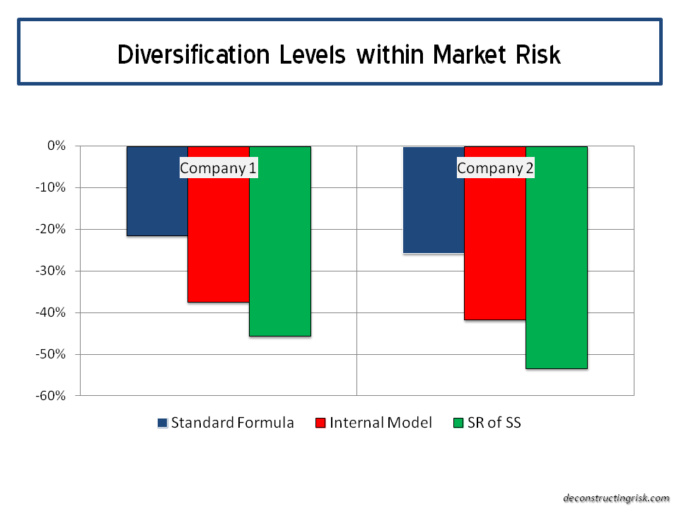
Diversification within the life underwriting risk module can also be significant (e.g. 40% to 50%) particularly where firms write significant mortality and longevity type exposures. Within the non-life underwriting risk module, diversification between the premium, reserving and catastrophe risks also add-up. The correlations in the standard formula on diversification between business classes vary between 25% and 50%.

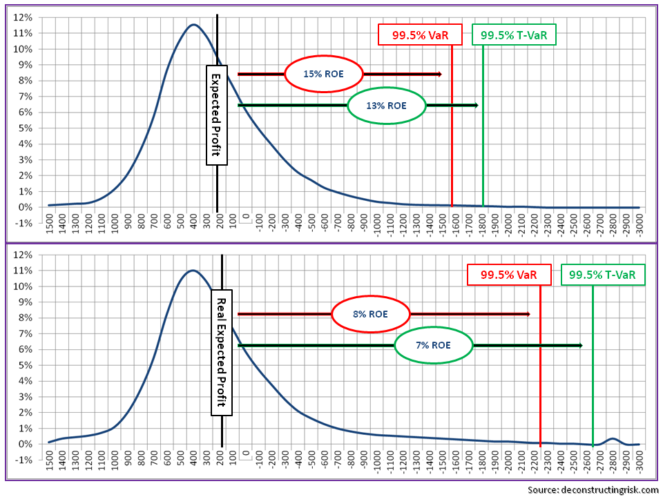
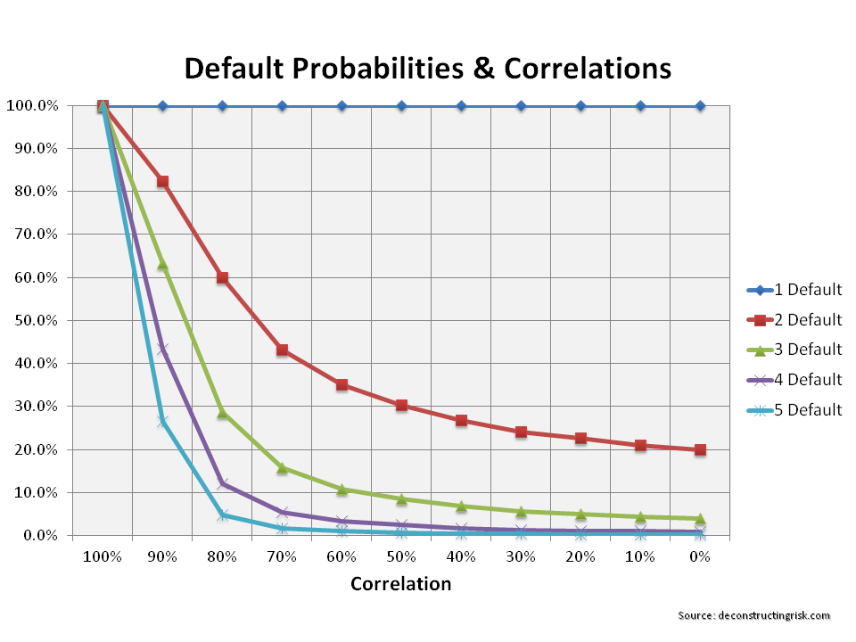
By way of a thought experiment, I constructed a non-life portfolio made up of five business classes (X1 to X5) with varying risk profiles (each class set with a return on equity expectation of between 10% and 12% at a capital level of 1 in 500 or 99.8% confidence level for each), as the graph below shows. Although many aggregate profiles may reflect ROEs of 10% to 12%, in my view, business classes in the current market are likely to have a more skewed profile around that range.

click to enlargeSample Insurance Portfolio Profile

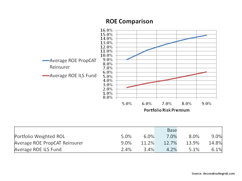
I then aggregated the business classes at varying correlations (simple point correlations in the random variable generator before the imposition of the differing distributions) and added a net expense load of 5% across the portfolio (bringing the expected combined ratio from 90% to 95% for the portfolio). The different resulting portfolio ROEs for the different correlation levels shows the impact of each assumption, as below.

click to enlargePortfolio Risk Profile various correlations

The experiment shows that a reasonably diverse portfolio that can be expected to produce a risk adjusted ROE of between 14% and 12% (again at a 1 in 500 level)with correlations assumed at between 25% and 50% amongst the underlying business classes. If however, the correlations are between 75% and 100% then the same portfolio is only producing risk adjusted ROEs of between 10% and 4%.

As correlations tend to increase dramatically in stress situations, it highlights the dangers of overtly generous diversification assumptions and for me it illustrates the need to be wary of firms that claim divine diversification.

Stressing the scenario testing

Scenario and stress testing by financial regulators has become a common supervisory tool since the financial crisis. The EU, the US and the UK all now regularly stress their banks using detailed adverse scenarios. In a recent presentation, Moody’s Analytics illustrated the variation in some of the metrics in the adverse scenarios used in recent tests by regulators, as per the graphic below of the peak to trough fall in real GDP.

click to enlargeBanking Stress Tests

Many commentators have criticized these tests for their inconsistency and flawed methodology while pointing out the political conflict many regulators with responsibility for financial stability have. They cannot be seen to be promoting a draconian scenario for stress testing on the one hand whilst assuring markets of the stability of the system on the other hand.

The EU tests have particularly had a credibility problem given the political difficulties in really stressing possible scenarios (hello, a Euro break-up?). An article last year by Morris Goldstein stated:

“By refusing to include a rigorous leverage ratio test, by allowing banks to artificially inflate bank capital, by engaging in wholesale monkey business with tax deferred assets, and also by ruling out a deflation scenario, the ECB produced estimates of the aggregate capital shortfall and a country pattern of bank failures that are not believable.”

In a report from the Adam Smith Institute in July, Kevin Dowd (a vocal critic of the regulator’s approach) stated that the Bank of England’s 2014 tests were lacking in credibility and “that the Bank’s risk models are worse than useless because they give false risk comfort”. Dowd points to the US where the annual Comprehensive Capital Assessment and Review (CCAR) tests have been supplemented by the DFAST tests mandated under Dodd Frank (these use a more standard approach to provide relative tests between banks). In the US, the whole process has been turned into a vast and expensive industry with consultants (many of them ex-regulators!) making a fortune on ever increasing compliance requirements. The end result may be that the original objectives have been somewhat lost.

According to a report from a duo of Columba University professors, banks have learned to game the system whereby “outcomes have become more predictable and therefore arguably less informative”. The worry here is that, to ensure a consistent application across the sector, regulators have been captured by their models and are perpetuating group think by dictating “good” and “bad” business models. Whatever about the dangers of the free market dictating optimal business models (and Lord knows there’s plenty of evidence on that subject!!), relying on regulators to do so is, well, scary.

To my way of thinking, the underlying issue here results from the systemic “too big to fail” nature of many regulated firms. Capitalism is (supposedly!) based upon punishing imprudent risk taking through the threat of bankruptcy and therefore we should be encouraging a diverse range of business models with sensible sizes that don’t, individually or in clusters, threaten financial stability.

On the merits of using stress testing for banks, Dowd quipped that “it is surely better to have no radar at all than a blind one that no-one can rely upon” and concluded that the Bank of England should, rather harshly in my view, scrap the whole process. Although I agree with many of the criticisms, I think the process does have merit. To be fair, many regulators understand the limitations of the approach. Recently Deputy Governor Jon Cunliffe of the Bank of England admitted the fragilities of some of their testing and stated that “a development of this approach would be to use stress testing more counter-cyclically”.

The insurance sector, particularly the non-life sector, has a longer history with stress and scenario testing. Lloyds of London has long required its syndicates to run mandatory realistic disaster scenarios (RDS), primarily focussed on known natural and man-made events. The most recent RDS are set out in the exhibit below.

click to enlargeLloyds Realistic Disaster Scenarios 2015

A valid criticism of the RDS approach is that insurers know what to expect and are therefore able to game the system. Risk models such as the commercial catastrophe models sold by firms like RMS and AIR have proven ever adapt at running historical or theoretical scenarios through today’s modern exposures to get estimates of losses to insurers. The difficulty comes in assigning probabilities to known natural events where the historical data is only really reliable for the past 100 years or so and where man-made events in the modern world, such as terrorism or cyber risks, are virtually impossible to predict. I previously highlighted some of the concerns on the methodology used in many models (e.g. on correlation here and VaR here) used to assess insurance capital which have now been embedded into the new European regulatory framework Solvency II, calibrated at a 1-in-200 year level.

The Prudential Regulatory Authority (PRA), now part of the Bank of England, detailed a set of scenarios last month to stress test its non-life insurance sector in 2015. The detail of these tests is summarised in the exhibit below.

click to enlargePRA General Insurance Stress Test 2015

Robert Childs, the chairman of the Hiscox group, raised some eye brows by saying the PRA tests did not go far enough and called for a war game type exercise to see “how a serious catastrophe may play out”. Childs proposed that such an exercise would mean that regulators would have the confidence in industry to get on with dealing with the aftermath of any such catastrophe without undue fussing from the authorities.

An efficient insurance sector is important to economic growth and development by facilitating trade and commerce through risk mitigation and dispersion, thereby allowing firms to more effectively allocate capital to productive means. Too much “fussing” by regulators through overly conservative capital requirements, maybe resulting from overtly pessimistic stress tests, can result in economic growth being impinged by excess cost. However, given the movement globally towards larger insurers, which in my view will accelerate under Solvency II given its unrestricted credit for diversification, the regulator’s focus on financial stability and the experiences in banking mean that fussy regulation will be in vogue for some time to come.

The scenarios selected by the PRA are interesting in that the focus for known natural catastrophes is on a frequency of large events as opposed to an emphasis on severity in the Lloyds’ RDS. It’s arguable that the probability of the 2 major European storms in one year or 3 US storms in one year is significantly more remote than the 1 in 200 probability level at which capital is set under Solvency II. One of the more interesting scenarios is the reverse stress test such that the firm becomes unviable. I am sure many firms will select a combination of events with an implied probability of all occurring with one year so remote as to be impossible. Or select some ultra extreme events such as the Cumbre Vieja mega-tsunami (as per this post). A lack of imagination in looking at different scenarios would be a pity as good risk management should be open to really testing portfolios rather than running through the same old known events.

New scenarios are constantly being suggested by researchers. Swiss Re recently published a paper on a reoccurrence of the New Madrid cluster of earthquakes of 1811/1812 which they estimated could result in $300 billion of losses of which 50% would be insured (breakdown as per the exhibit below). Swiss Re estimates the probability of such an event at 1 in 500 years or roughly a 10% chance of occurrence within the next 50 years.

click to enlarge1811 New Madrid Earthquakes repeated

Another interesting scenario, developed by the University of Cambridge and Lloyds, which is technologically possible, is a cyber attack on the US power grid (in this report). There have been a growing number of cases of hacking into power grids in the US and Europe which make this scenario ever more real. The authors estimate the event at a 1 in 200 year probability and detail three scenarios (S1, S2, and the extreme X1) with insured losses ranging from $20 billion to $70 billion, as per the exhibit below. These figures are far greater than the probable maximum loss (PML) estimated for the sector by a March UK industry report (as per this post).

click to enlargeCyber Blackout Scenario

I think it will be a very long time before any insurer willingly publishes the results of scenarios that could cause it to be in financial difficulty. I may be naive but I think that is a pity because insurance is a risk business and increased transparency could only lead to more efficient capital allocations across the sector. Everybody claiming that they can survive any foreseeable event up to a notional probability of occurrence (such as 1 in 200 years) can only lead to misplaced solace. History shows us that, in the real world, risk has a habit of surprising, and not in a good way. Imaginative stress and scenario testing, performed in an efficient and transparent way, may help to lessen the surprise. Nothing however can change the fact that the “unknown unknowns” will always remain.

Tails of VaR

In an opinion piece in the FT in 2008, Alan Greenspan stated that any risk model is “an abstraction from the full detail of the real world”. He talked about never being able to anticipate discontinuities in financial markets, unknown unknowns if you like. It is therefore depressing to see articles talk about the “VaR shock” that resulted in the Swissie from the decision of the Swiss National Bank (SNB) to lift the cap on its FX rate on the 15th of January (examples here from the Economist and here in the FTAlphaVille). If traders and banks are parameterising their models from periods of unrepresentative low volatility or from periods when artificial central bank caps are in place, then I worry that they are not even adequately considering known unknowns, let alone unknown unknowns. Have we learned nothing?

Of course, anybody with a brain knows (that excludes traders and bankers then!) of the weaknesses in the value-at-risk measure so beloved in modern risk management (see Nassim Taleb and Barry Schachter quotes from the mid 1990s on Quotes page). I tend to agree with David Einhorn when, in 2008, he compared the metric as being like “an airbag that works all the time, except when you have a car accident“.  A piece in the New York Times by Joe Nocera from 2009 is worth a read to remind oneself of the sad topic.

This brings me to the insurance sector. European insurance regulation is moving rapidly towards risk based capital with VaR and T-VaR at its heart. Solvency II calibrates capital at 99.5% VaR whilst the Swiss Solvency Test is at 99% T-VaR (which is approximately equal to 99.5%VaR). The specialty insurance and reinsurance sector is currently going through a frenzy of deals due to pricing and over-capitalisation pressures. The recently announced Partner/AXIS deal follows hot on the heels of XL/Catlin and RenRe/Platinum merger announcements. Indeed, it’s beginning to look like the closing hours of a swinger’s party with a grab for the bowl of keys! Despite the trend being unattractive to investors, it highlights the need to take out capacity and overhead expenses for the sector.

I have posted previously on the impact of reduced pricing on risk profiles, shifting and fattening distributions. The graphic below is the result of an exercise in trying to reflect where I think the market is going for some businesses in the market today. Taking previously published distributions (as per this post), I estimated a “base” profile (I prefer them with profits and losses left to right) of a phantom specialty re/insurer. To illustrate the impact of the current market conditions, I then fattened the tail to account for the dilution of terms and conditions (effectively reducing risk adjusted premia further without having a visible impact on profits in a low loss environment). I also added risks outside of the 99.5%VaR/99%T-VaR regulatory levels whilst increasing the profit profile to reflect an increase in risk appetite to reflect pressures to maintain target profits. This resulted in a decrease in expected profit of approx. 20% and an increase in the 99.5%VaR and 99.5%T-VaR of 45% and 50% respectively. The impact on ROEs (being expected profit divided by capital at 99.5%VaR or T-VaR) shows that a headline 15% can quickly deteriorate to a 7-8% due to loosening of T&Cs and the addition of some tail risk.

click to enlargeTails of VaR

For what it is worth, T-VaR (despite its shortfalls) is my preferred metric over VaR given its relative superior measurement of tail risk and the 99.5%T-VaR is where I would prefer to analyse firms to take account of accumulating downside risks.

The above exercise reflects where I suspect the market is headed through 2015 and into 2016 (more risky profiles, lower operating ROEs). As Solvency II will come in from 2016, introducing the deeply flawed VaR metric at this stage in the market may prove to be inappropriate timing, especially if too much reliance is placed upon VaR models by investors and regulators. The “full detail of the real world” today and in the future is where the focus of such stakeholders should be, with much less emphasis on what the models, calibrated on what came before, say.

Confounding correlation

Nassim Nicholas Taleb, the dark knight or rather the black swan himself, said that “anything that relies on correlation is charlatanism”.  I am currently reading the excellent “The signal and the noise” by Nate Silver. In Chapter 1 of the book he has a nice piece on CDOs as an example of a “catastrophic failure of prediction” where he points to certain CDO AAA tranches which were rated on an assumption of a 0.12% default rate and which eventually resulted in an actual rate of 28%, an error factor of over 200 times!.

Silver cites a simplified CDO example of 5 risks used by his friend Anil Kashyap in the University of Chicago to demonstrate the difference in default rate if the 5 risks are assumed to be totally independent and dependent.  It got me thinking as to how such a simplified example could illustrate the impact of applied correlation assumptions. Correlation between core variables are critical to many financial models and are commonly used in most credit models and will be a core feature in insurance internal models (which under Solvency II will be used to calculate a firms own regulatory solvency requirements).

So I set up a simple model (all of my models are generally so) of 5 risks and looked at the impact of varying correlation from 100% to 0% (i.e. totally dependent to independent) between each risk. The model assumes a 20% probability of default for each risk and the results, based upon 250,000 simulations, are presented in the graph below. What it does show is that even at a high level of correlation (e.g. 90%) the impact is considerable.

click to enlarge5 risk pool with correlations from 100% to 0%

The graph below shows the default probabilities as a percentage of the totally dependent levels (i.e 20% for each of the 5 risks). In effect it shows the level of diversification that will result from varying correlation from 0% to 100%. It underlines how misestimating correlation can confound model results.

click to enlargeDefault probabilities & correlations

ILS Fund versus PropertyCat Reinsurer ROEs

Regular readers will know that I have queried how insurance-linked securities (ILS) funds, currently so popular with pensions funds, can produce a return on equity that is superior to that of a diversified property catastrophe reinsurer given that the reinsurer only has to hold a faction of its aggregate limit issued as risk based capital whereas all of the limits in ILS are collaterised. The recent FT article which contained some interesting commentary from John Seo of Fermat Capital Management got me thinking about this subject again. John Seo referred to the cost advantage of ILS funds and asserted that reinsurers staffed with overpaid executives “can grow again, but only after you lay off two out of three people”. He damned the traditional sector with “these guys have been so uncreative, they have been living off earthquake and hurricane risks that are not that hard to underwrite.

Now, far be it from me to defend the offshore chino loving reinsurance executives with a propensity for large salaries and low taxation. However, I still can’t see that the “excessive” overheads John Seo refers to could offset the capital advantage that a traditional property catastrophe reinsurer would have over ILS collateral requirements.

I understood the concept of ILS structures that provided blocks of capacity at higher layers, backed by high quality assets, which could (and did until recently) command a higher price than the traditional market. Purchasers of collaterised coverage could justify paying a premium over traditional coverage by way of large limits on offer and a lower counterparty credit risk (whilst lowering concentration risk to the market leading reinsurers). This made perfect sense to me and provided a complementary, yet different, product to that offered by traditional reinsurers. However, we are now in a situation whereby such collaterised reinsurance providers may be moving to compete directly with traditional coverage on price and attachment.

To satisfy my unease around the inconsistency in equity returns, I decided to do some simple testing. I set up a model of a reasonably diversified portfolio of 8 peak catastrophic risks (4 US and 4 international wind and quake peak perils). The portfolio broadly reflects the market and is split 60:40 US:International by exposure and 70:30 by premium. Using aggregate exceedance probability (EP) curves for each of the main 8 perils based off extrapolated industry losses as a percentage of limits offered across standard return periods, the model is set up to test differing risk premiums (i.e. ROL) for each of the 8 perils in the portfolio and their returns.  For the sake of simplicity, zero correlations were assumed between the 8 perils.

The first main assumption in the model is the level of risk based capital needed by the property catastrophe reinsurer to compete against the ILS fund. Reviewing some of the Bermudian property catastrophe players, equity (common & preferred) varies between 280% and 340% of risk premiums (net of retrocessions). Where debt is also included, ratios of up to 400% of net written premiums can be seen. However, the objective is to test different premium levels and therefore setting capital levels as a function of premiums distorts the results. As reinsurer’s capital levels are now commonly assessed on the basis of stressed economic scenarios (e.g. PMLs as % of capital), I did some modelling and concluded that a reasonable capital assumption for the reinsurer to be accepted is the level required at a 99.99th percentile or a 1 in 10,000 return period (the graph below shows the distribution assumed). As the graph below illustrates, this equates to a net combined ratio (net includes all expenses) of the reinsurer of approximately 450% for the average risk premium assumed in the base scenario (the combined ratio at the 99.99th level will change as the average portfolio risk premium changes).

click to enlargePropCAT Reinsurer Combined Ratio Distribution

So with the limit profile of the portfolio is set to broadly match the market, risk premiums per peril were also set according to market rates such that the average risk premium from the portfolio was 700 bps in a base scenario (again broadly where I understand the property catastrophe market is currently at).

Reviewing some of the actual figures from property catastrophe reinsurer’s published accounts, the next important assumption is that the reinsurer’s costs are made up of 10% acquisition costs and 20% overhead (the overhead assumption is a bit above the actual rates seen by I am going high to reinforce Mr Seo’s point about greedy reinsurance executives!) thereby reducing risk premiums by 30%. For the ILS fund, the model assumes a combined acquisition and overhead cost of just 10% (this may also be too light as many ILS funds are now sourcing some of their business through brokers and many reinsurance fund managers share the greedy habits of the traditional market!).

The results below show the average simulated returns for a reinsurer and an ILS fund writing the same portfolio with the expense levels as detailed above (i.e 30% versus 10%), and with different capital levels (reinsurer at 99.99th percentile and the ILS fund with capital equal to the limits issued). It’s important to stress that the figures below do not included investment income so historical operating ROEs from property catastrophe reinsurers are not directly comparable.

click to enlargePropCAT Reinsurer & ILS Fund ROE Comparison

So, the conclusion of the analysis re-enforces my initial argument that the costs savings cannot compensate for the leveraged nature of a reinsurer’s business model compared to the ILS fully funded model. However, this is a simplistic comparison. Why would a purchaser not go with a fully funded ILS provider if the product on offer was exactly the same as that of a reinsurer? As outlined above, both risk providers serve different needs and, as yet, are not full on competitors (although this may be the direction of the changes underway in the market currently).

Also, many ILS funds likely do use some form of leverage in their business model whether by way of debt or retrocession facilities. And competition from the ILS market is making the traditional market look at its overhead and how it can become more cost efficient. So it is likely that both business models will adapt and converge (indeed, many reinsurers are now also ILS managers).

Notwithstanding these issues, I can’t help conclude that (for some reason) our pension funds are the losers here by preferring the lower returns of an ILS fund sold to them by investment bankers than the higher returns on offer from simply owning the equity of a reinsurer (admittedly without the same operational risk profile). Innovative or just cheap risk premia? Go figure.